Off Policy Prediction and Control with Approximation

• The main issue is guaranteeing convergence from methods that extend Temporal Difference Learning methods to use semi gradient descent.
• Another issue is that the distribution of updates in the off-policy case is not according to the on-policy distribution.
  • One approach to this is to apply Importance Sampling.

Semi-Gradient Methods §

• These methods address how we change update targets for off-policy approximation.
• They may diverge, but they are simple and stable, and asymptotically unbiased for the tabular case.
• We will make use of the per step importance sampling ratio as an additional weight to the gradient
  • For semi-gradient Expected SARSA, even though we do not use importance sampling in the tabular case, in the functional approximation case, we use importance sampling to give weight to certain actions.
  • Note that for -step bootstrapping methods, we make use of as weights.

Divergence §

• Divergence arises when we have all three of the following (and yet we cannot give them up for performance reasons).

  • Function approximation — generalizing state space with smaller representations.
  • Bootstrapping - updating using estimates rather than actual values
  • Off-policy training - particularly since the behavior policy may choose actions that the target policy would never.

• Baird’s counterexample shows that even certain systems can be unstable, regardless if we use off-policy with approximation or the tabular case, for as long as we do not use the on-policy distribution.

  • The instability arises because in a sense, the counterexample is overparameterized, and it has infinitely many solutions. The solution picked by the algorithm is dependent on how we initialize the values of each state (and also, how we sample from them using the behavior policy and perform updates on them).

• To prevent divergence we may use special methods — stability is guaranteed for methods (averagers) that do not extrapolate from observed targets.

• We also have to contend with the high variance of off-policy algorithms. One way to do this is by having a small enough learning styles.

• Another way is to allow the target policy be determined in part by the behavior policy. One is never different from the other.

Gradient Descent Algorithms §

Residual Gradient Algorithm §

• The goal is to minimize the Bellman Error

• A similar “goal” is the mean square TD error defined as

  Where is the behavioral policy, and is the importance sampling constant. This goal is naive because the policy that minimizes TDE is not necessarily the best policy.

• The residual gradient algorithm is defined as follows

  • The problem with this is because we use in two different expectations, we have a biased estimator (for stochastic environments).
  • One way to remedy this problem is to obtain two independent samples of the next state . (assuming interaction with a simulated environment)
  • Disadvantages:
    • It is much slower than semi-gradient methods.
    • It converges to the wrong value functions.
    • The Bellman Error is not learnable.

Gradient-TD Methods §

• The goal is to use SGD to minimize PBE.

• Let be the distribution of states visited under the behavior policy.

• The gradient of PBE is obtained as

• We can store some estimate, specifically the product of the second and third terms. In fact, this is just the analytical solution to the linear supervised problem, so the goal can then become minimizing Least Mean Square.

• GTD-2 is one such variant that performs the update as

• GTD-0 (also called with gradient correction or TDC) improves on GTD-2 by doing more analytic steps before substitution.

• The goal of GTD-0 is to learn a parameter such that even from data that is due to following another policy.

Emphatic TD Methods §

• The idea is to reweight the states to emphasize some and de-emphasize others so as to return the distribution of updates to the on-line policy distribution.

• We make use of pseudo-termination — termination such as discounting, that does not affect the sequence of state transitions, but does affect the learning process.

• We define the algorithm as follows

Where is the interest and is the emphasis, initialized to

Other Algorithms §

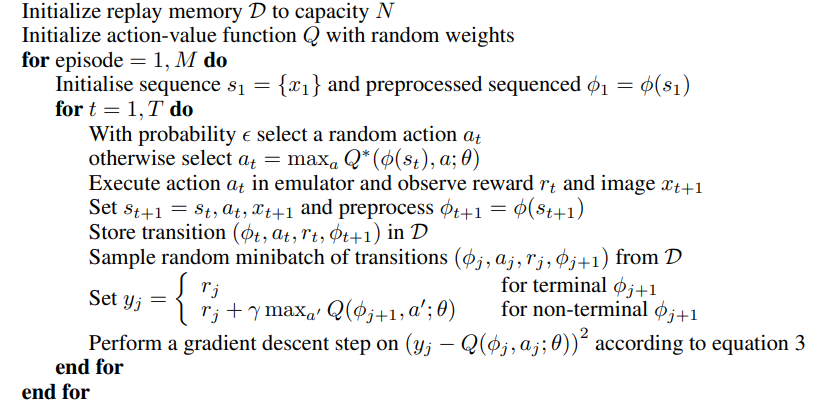
DQN §

• Generalizes Q-learning to a functional approximation setting, but applying innovations to stabilize it¹
• A Q-Network is a Neural Network trained to minimize the following loss function
  Where
  refers to the behavior distribution.
  • Note: The targets depend on the current weights. The gradient is derived as:
• Experience Replay - All episode steps are stored in a growing dataset of replay memory . We then sample a minibatch from the replay memory during updates.
  • It has the following advantages:
    • It reduces non-stationarity
    • Random sampling reduces variance by decorrelating the data (consecutive episode steps are correlated)
    • It prevents training converging to local minima which can happen when the learning is too dependent on the behavior distribution. Experience replay lets us average out the behavior distribution.
  • However, on its own:
    • It uses more memory and computation
    • It requires an off-policy learning algorithm that can update from data generated by an older policy. ²
  • Actions are then selected via an -greedy policy.

DQN with Experience Learning. Taken from Minh (2013)

Links §

• Sutton and Barto Ch. 11

  • 11.1 - more on semi-gradient variants to off-policy methods.
  • 11.2 - discusses Baird’s counterexample and the divergence of off-policy methods.
  • 11.7 - more on Gradient-TD methods.

• Function Approximation in Reinforcement Learning

• Temporal Difference Learning - more on Off-Policy learning techniques.

• A Unified View on Reinforcement Learning Approaches - more on off-policy

Footnotes §

1. Mnih, et al. (2013). Playing Atari with Deep Reinforcement Learning ↩

2. Mnih, et al. Asynchronous methods for deep reinforcement learning. ICML. 2016. ↩