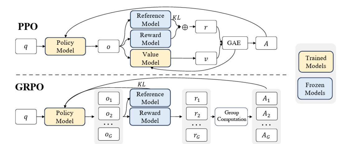
GRPO
- Group Relative Policy Optimization 1
- It builds upon PPO while optimizing for memory usage by removing a Value Model.
- Instead of a Value Model that acts as a critic, use the average reward of multiple sample model outputs using the same input.
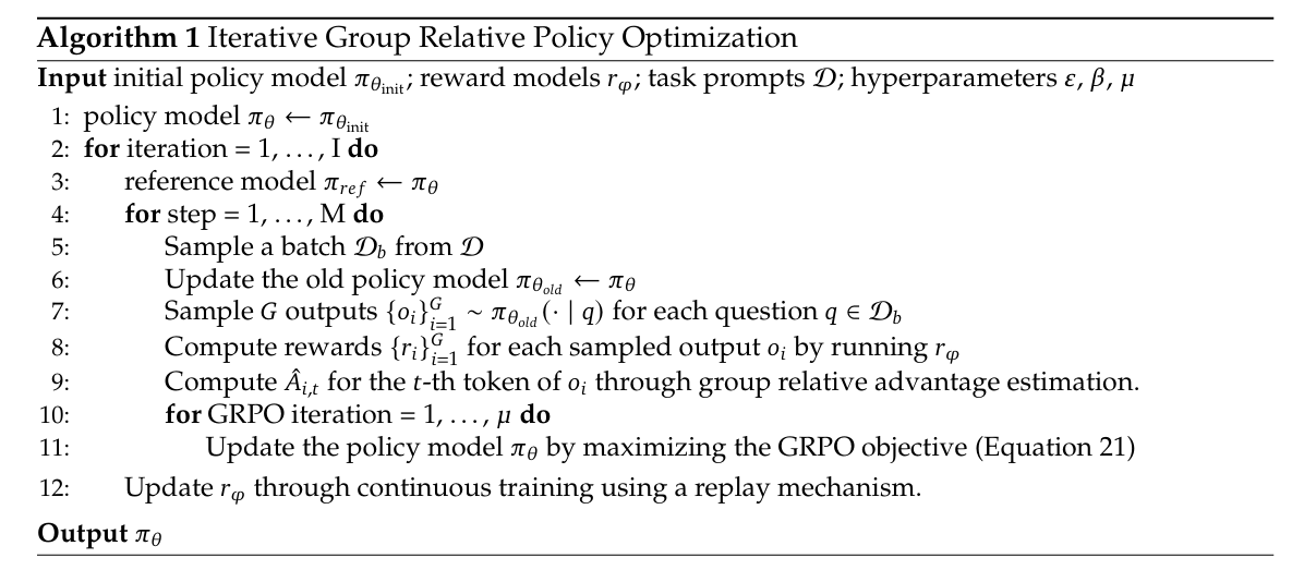
- The objective is then formulated as follows (see PPO-CLIP). Let
be the output group sampled from with as the output (which can be a sequence of outputs over time) and the fixed input. Then With the probability ratio being given byAnd advantagecalculated based on relative rewards of outputs inside each group only. - We use Schulman’s approximation to estimate the KL Divergence
- Outcome Supervision provides the normalized reward at the end of each output. This is done as follows. For outputs
, a reward model scores these 2 to yield . The rewards are normalized and the advantage is given as the normalized reward. That is And - Policy Supervision can also be done to provide rewards at the end of each reasoning step In this case,
where is the end token index of the -th step and is the total number of steps. The total reward is then given by - To make GRPO Iterative, we can generate new training sets for the reward model based on the sampling results from the policy model. We could then train the reward model via a replay mechanism.
PPO
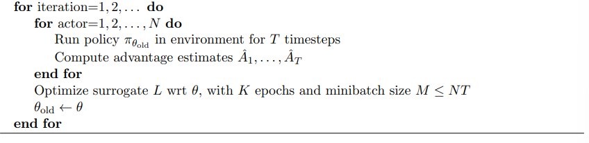
- Proximal Policy Optimization 3. These alternate between sampling data through interaction with the environment, and optimizing a “surrogate” objective function using SGD.
- The goal is scalability since TRPO is complicated and not good for noisy architectures.
- The assumed objective by default is PPO-CLIP.
PPO-CLIP
-
It introduces the clipped surrogate objective. Let
denote the probability ratio The surrogate objective becomes
The first term in the min function above is the same objective as TRPO. The second modifies the surrogate objective by clipping the probability ratio, removing the incentive for moving
outside the interval . This is to make things more stable. The final bound given by the loss function above is a lower bound (i.e., a pessimistic bound) on the unclipped objective.
Thus, we ignore
when it makes the objective better and include it when it makes the objective worse.
PPO-KL
- An alternative is KL Penalization — we use a penalty on the KL divergence and adapt the penalty based on a targeted KL divergence. This can be done by alternating between the following
-
Use Minibatch SGD to optimize
-
Compute
- If
, then - If
, then .
- If
-
We use the updated
for the next policy update. The constants are magic but the algorithm is not sensitive to them. -
Note that we can alternatively use the backward version which involves
. This yields no difference. -
Techniques presented here may be combined with the loss function above. For example , introducing entropy loss
. as a penalty term, or using Experience replay. -
Using entropy loss gives us this loss function
-
Failure Modes
-
4 revisited PPO to examine two common design choices.
- The clipped probability ratio
- Parameterizing the policy action space by a continuous Gaussian or a discrete softmax.
-
The following happens in standard PPO
- When we have reward signals with bounded support This is problematic when the reward causes the policy to end up in regions with low rewards which would allow it to recover.
- This is common when we have unknown action boundaries or sparse rewards.
- High dimensional discrete action spaces. This causes PPO to get stuck at suboptimal actions.
- Locally optimal actions close to initialization. PPO is sensitive to initialization and will converge to locally optimal actions close to initialization.
- When we have reward signals with bounded support This is problematic when the reward causes the policy to end up in regions with low rewards which would allow it to recover.
-
The following are the proposed solutions
- Use KL regularization instead of the usual clipped loss. That is, we perform. This solves failure modes 1 and 2.
- KL forces large steps to have a large opposite gradient from the KL penalty so that we do not immediately leave the trust region.
- Instead of a Gaussian, use a Beta distribution as a parameterization for continuous action spaces. This solves failure modes 1 and 3
- Compared to Gaussian policies where actions in the tails are given more importance, Beta policies give tails lower importance. All actions are weighted evenly
- Additionally it is easier to integrate a uniform prior on a Beta distribution by setting
. - It eliminates the bias towards the boundaries in truncated Gaussian on bounded action spaces.
- Use KL regularization instead of the usual clipped loss. That is, we perform. This solves failure modes 1 and 2.
PPG
-
Phasic Policy Gradient 5 extends PPO to have two separate training phases for policy and value functions. This leads to significant improvements on sample efficiency .
-
It provides an alternative to sharing network parameters which have the disadvantages of:
- Being hard to balance so that competing objectives do not interfere with each other. This interference can impact performance.
- Enforcing a hard restriction that policy and value function objectives are trained on the same data subject to the same sample reuse. Value functions tend to tolerate a higher level of sample reuse
-
In PPG, we have disjoint policy and value networks.
- The policy network has policy
and auxiliary value head . - The value network has a value head of
- The policy network has policy
-
PPG introduces two training phases. Learning proceeds by alternating between them.
-
Policy Phase - train the agent with PPO using
for the policy, and for the value function of the policy network -
Auxiliary Phase - distill features from the value function into the policy network for training future policy phases. We use the following loss function
Where
is the policy before the auxiliary begins. is a hyperparameter controlling the tradeoff between the auxiliary objective and the original policy is the auxiliary objective, which can be anything. The paper gives the following
-
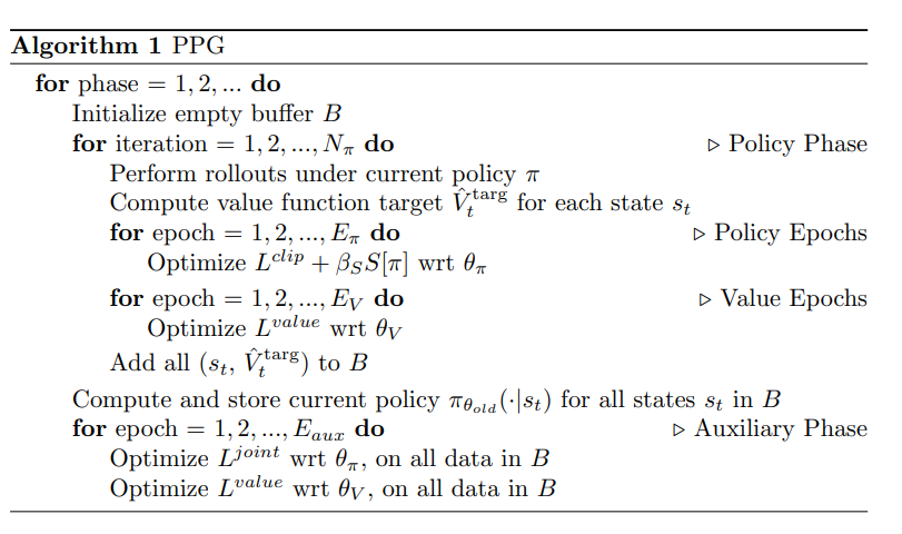
- In the figure
controls the number of policy updates performed in each policy phase controls sample reuse for the policy controls sample reuse for the true value function controls the sample reuse during the auxiliary phase. We increase this to increase sample reuse for the value function.
ACKTR
-
Actor Critic using Kronecker-factored trust region 6
-
It builds upon TRPO. It Proposes to use the Kronecker-factored approximation curvature (K-FAC) to perform the gradient updates for both the actor and the critic.
-
We make use of natural gradients rather than our usual gradients. This means that our step sizes are based on the KL divergence from the current network.
-
KFAC approximates the gradient using Kronecker products between smaller matrices
TRPO
-
Trust Region Policy Optimization 7. It aims to optimize large non-linear policies (i.e., those that use neural networks) by using a surrogate loss function. In particular, this is based on the KL divergence
-
For convenience, we let
-
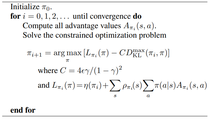
The notes here are helpful as a background for why we have TRPO. The theoretical bound is then given for old policy
and new policy as -
This gives the following algorithm for policy improvement.
-
TRPO reframes the objective as maximizing
(see above). However, we use the approximation . More specifically, we can use the Importance Sampling ratio and replace the advantage with . That is, the objective becomes -
In practice, we do not use
because this gives small step sizes. Instead we maximize subject to the constraint that for threshold . This is the trust region constraint
-
The trust region constraint guarantees that old and new policies do not diverge too much while guaranteeing monotonic improvement. 8
-
The
value can be replaced with an empirical estimate. - Single Path - Estimates for
comes from a single trajectory - Vine -Given a single trajectory, sample states, and from each sampled state, sample actions. From there, perform a rollout and estimate
from the rollout trajectories. - Vine gives a better estimate with lower variance at the cost of requiring more calls as well as not being feasible for systems where “undoing” is not possible .
- Single Path - Estimates for
Footnotes
-
Shao et al. (2024) DeepSeekMath: Pushing the Limits of Mathematical Reasoning in Open Language Models ↩
-
Keep in mind this was written in an LLM context. In practice, if we don’t have a reward model for scoring, refer to the resulting rewards via the environment dynamics ↩
-
Schulman et al. (2017) Proximal Policy Optimization Algorithms ↩
-
Hsu, Mendler-Dummer, and Hardt (2020) Revisiting Design Choices in Proximal Policy Optimization ↩
-
Cobbe et al. (2020) Phasic Policy Gradient ↩
-
Wu et al. (2017) Scalable trust-region method for deep reinforcement learning using Kronecker-factored approximation ↩
-
Schulman et al. (2015) Trust Region Policy Optimization ↩
-
The KL divergence makes this intuitive since it measures the similarity between two probability distributions, and recall that policies are probability distributions. ↩