Pathologies of Deep Learning

Learning Variants §

• Classification involves identifying the group that an entity belongs in given its features. It has important variants.

  • Binary - only two labels
  • Multiclass - more than two labels
  • Multilabel - can predict more than two labels.

• In batch learning, we have access to the features and the labels, which we may use to train a model. When we then deploy this model, we no longer retrain or update the model barring extreme circumstances (and we do updates in batches).

• In online learning we have data points that arrive one sample at a time. More specifically, we formulate an estimation and only when we have done this can we observe .

  We follow a cycle where we have to continuously improve the model given new observations

  • The bandit problem is a special variation wherein instead of having a continuously parameterized model , we have a finite number of actions that we can take and we must allocate our resources to minimize loss.

Distribution Shift §

• A distribution shift pertains to a problem in making a model wherein the assumption that the distribution of the problem domain being stationary does not hold.

Covariate Shift §

• Covariate Shift - involves a shift in the distribution of the features but not the labeling function. More specifically, changes.

• It is a natural assumption when we believe causes .

• Assume: that each data has a nonzero probability of occurring during training time.

• We can mitigate as follows. Let be the source distribution and the target. By definition did not change.

  We correct using the risk identity but using the a modified Empirical risk instead

  LetSo that the empirical risk becomes All that is left is to actually estimate the term. This will require sampling from both and . ¹

• An alternative to this is to use logistic regression to distinguish between samples from one distribution to another. This means we modify

Label Shift §

• In Label Shift we assume that the distribution of label changes but not .

• It is a natural assumption when causes .

• We can use something similar to how we solved Covariate Shift except we have to estimate the target label distribution and the confusion matrix using the validation set (from the same distribution as the training set).

• Assume:

  • We have a classifier that is already accurate on the training distribution.
  • The target distribution only contains categories we have seen before.
  • We are actually dealing with label shift and nothing else.

• Perform the following procedure

1. Obtain the classifier model and obtain the confusion matrix as above.
2. Average all the model’s predictions at test time together, yielding mean model outputs where the -the element is the fraction of total predictions on the test set where our model predicted .
3. Solve for the system of linear equations:
4. Estimate the distribution by looking at the source data labels.
5. Obtain as shown above and minimize the empirical risk weighted with .

Concept Shift §

• Concept Shift is a form of distribution shift that arises when the very definition of the labels changes.

• We can mitigate this by gradually updating the Model and making it adapt to any changes in data. We do not need to retrain our models.

• Internal Covariate Shift refers to a supposed phenomenon that occurs within very deep models. The inputs of the intermediate layers vary in magnitude and can hamper the convergence of the model.

• Environment Shift - happens when a model influences an environment that can also adapt to the actions of the model.

Nonstationarity §

• A stationary distribution is one where the unconditional joint probability distribution does not change when shifted in time. Any statistical measures or dynamics do not change.
• Non-stationary distributions are a form of distribution shift where the distribution changes slowly and the model is not adequately updated.

Generalization §

• Generalization gives counter intuitive results when it comes to deep learning

• Most deep learning modes can achieve arbitrarily low training error.

• Further gains in model performance (generalization) can only be obtained by reducing overfitting.

  This follows from (1) since we can make the training error arbitrarily small so minimizing the generalization gap boils down to reducing generalization error.

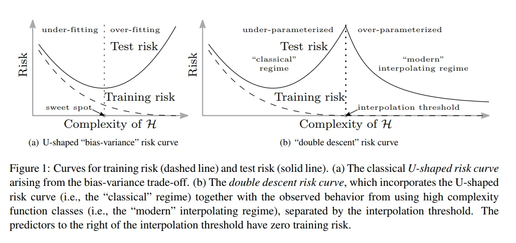
• Complexity != Overfitting. See Double Descent

• We cannot actually explain why a DNN generalizes.

• Regularization techniques do not improve the performance of the model (although they may help computation).

• Despite how we have parameters in a neural network, the neural network behaves more like a non-parametric model which perfectly interpolates between the training data. In some sense DNNs are more dependent on the training data and choice of inductive biases than any hyperparameters.

Double Descent §

• Double Descent pertains to a phenomenon where a model that is extremely simple (underparameterized) and a model that is extremely complex (overparameterized) will have high error, but a model whose number of parameters is about the same as the number of data points used to train it will have low error.
• Related to Bias Variance Tradeoff

Double Descent Illustration. Taken from evhub

Permutation Symmetry §

• Permutation Symmetry is an issue when it comes to training a neural network.

• In theory, all the parameters from one layer are indistinguishable from those of another layer. So it is possible to permute these parameters in such a way the order is different but the function is the same.

  So, if we initialized each parameter to have the same value, in forward propagation they will valuate to the same values, and in backpropagation they will have equal gradients meaning they did not update.

  Effectively, this means that our hidden layer would behave as if it were a single computational unit.

• We can mitigate permutation symmetry with proper parameter initialization A parameter initialization procedure determines how we initialize each parameter in the neural network.

Xavier Initialization §

• One example of a parameter initialization scheme is Xavier Initialization, wherein we initialize weights from a probability distribution with mean and variance .

• Consider the current layer and its previous layer which have been initialized by Xavier Initialization (with as its variance)

  Let be the inputs (size ) and be the weights of this layer. be the number of outputs of this layer.

  For simplicity, we will assume a lack of nonlinearities, so that the output is simply: .

  We can find the expectation and the variance as:

  We denote to be the function where we square all the components in the vector.

  One way to keep the variance fixed is to set but backpropagation means that we also have to do this for the next layer so we have to have , which would be impossible (especially since we don’t assume ).

  We loosen the condition and simply satisfy a mix of the two

  This is the variance that we choose to use for Xavier initialization. For the current layer, sample from a probability distribution where and

Gradients and Learning Rate §

• The Exploding Gradient Problem is an issue in deep learning. Because we perform successive multiplications, we may encounter gradients (and thus parameter updates) that are excessively large, which means each parameter drastically updates, and this can lead to the existing model being destroyed since we cannot achieve

• The Vanishing Gradient Problem is a problem in deep learning. Because we perform successive multiplications, we may encounter gradients (and thus parameter updates) that are excessively small, which means each parameter hardly updates.

  • Aside from the inherent numerical instability, this is influenced by the choice of activation functions.
  • For example, using sigmoid tends to cause gradients to vanih

• The learning rate is a hyperparameter that defines the step size at each iteration when moving towards the minimum of a loss function. Typically denoted .

  • Too low of a learning rate means the model gets stuck on local minima and will converge must slower.
  • Too high of a learning rate will jump over the minima

• One way to fix this is to use Residual Learning

Test Set Reuse §

• We must be careful when we reuse the test set for testing another model since we cannot guarantee that the next model will receive a misleading prediction score

Performance §

• Underfitting and overfitting are both concerns.

Links §

• Understanding Double Descent
• Neural Network
• Optimization Algorithms in Machine Learning

Footnotes §

1. This is similar in principle to Importance Sampling ↩