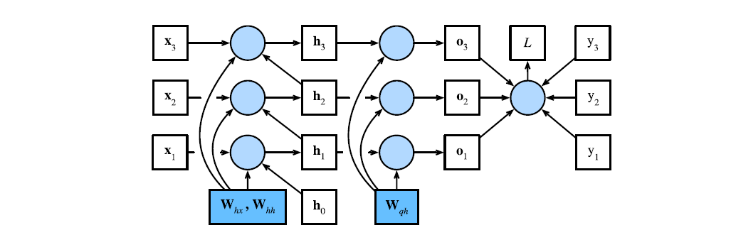
Backpropagation through Time

• Because of this training method, RNNs are susceptible to Vanishing and Exploding gradients.
• RNNs are also more susceptible to local optima.

Analysis of Gradients §

• Let be a hidden state be an input be an output for time step of some sequential data

  Also let , , be the weight parameters be the loss.

• By the recursion we have that

• The loss function can be evaluated as

BPTT flow. Image taken from Zhang et al.

• Performing BPTT will involve calculating

  Next, from the above we recall that . We have

  Next, we compute for . If then the chain rule simplifies since only depends on so

  If , then depends on via and . Now, by chain rule, we can recursively compute the gradient as

  And condensing the above by flattening the recursion, we may obtain

  Finally, we get

  And

• Note that is both numerically unstable and expensive to compute

Gradient Clipping §

• We can mitigate gradient issues in Backpropagation through time with Gradient Clipping.

• Assume we have an objective function that is Lipschitz continuous with constant

  We have by definition

  Updating parameter values using Gradient Descent means that we have for learning rate and gradient

  So that the objective function cannot change by more than the RHS of the inequality above.

  In Gradient Clipping, therefore, we limit .

• There are a few approaches to this

  • Limit the learning rate. The downside is that it will take longer for the model to train since we have a smaller learning rate. This is especially true if the gradient rarely blows up.

  • The Gradient Clipping Heuristic can be used especially if gradient values are rare.

    We project the gradient onto a ball of radius . That is, in the above, we set to be

    • This allows us to limit the effect of any given minibatch during training.

• One upside is that we mitigate the problems of exploding and vanishing gradients.

• One downside to clipping is that we limit the speed at which we reduce the values of our objective function.

• Another downside is that it is harder to analyze the side effects of applying this technique since we no longer follow the true gradient.

Truncated BPTT §

• Truncated BPTT is a variation of BPTT where, when applying the chain rule to the recurrence in an RNN, we stop the calculation once we reach where denotes a hidden state and denotes the corresponding weights.
• This leads to an approximation of the gradient
• The model becomes more stable since it focuses only on short term influences rather than long term consequences.

Randomized Truncated BPTT §

• Randomized Truncated BPTT extends Truncated BPTT.

• The algorithm initially follows truncated BPTT. However, after a certain point, we replace the calculation of with a random variable whose expectation matches that of the gradient.

• We do this with a sequence with predefined values . Where

  That is, we choose either a value or at time step , and also determines the probability of choosing .

  The effect is that we randomly truncate the calculation of the gradient, and at the same time we calculate a weighted sum of sequences where long sequences are appropriate overweighted.

  We then calculate the gradient as

Teacher Forcing §

• Teacher Forcing is a training technique which involves feeding the observed sequence values back to the RNN after each step. This forces the RNN to stay close to the ground truth sequence.
• Intuition: Rather than having the model commit mistakes that accumulate, for each entry in the sequence, we tell the model if it was correct, and regardless, we give it the correct answer.

Links §

• Recurrent Neural Network
• Differential Calculus
• Dive into Deep Learning by Zhang, Lipton, Li and Smola