The Evolution of Recurrent Neural Networks

Elman RNN §

• An Elman RNN is the most basic RNN architecture consisting only of recurrent layers and no more modifications.

Elman Network

LSTM §

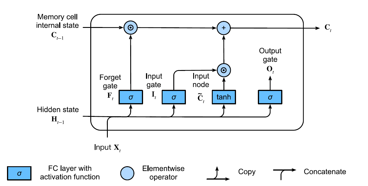
• Long Short Term Memory (LSTM) is an RNN architecture that improves over the Elman Network. We replace each recurrent node with an LSTM memory cell

• The term “long short-term memory” comes from the fact that standard recurrent neural networks have long term memory because of their weights. These weights change slowly during training, which encodes general knowledge about the data. RNNs also have short term memory because of their activations The LSTM model combines these two facets through memory cells.

• LSTMs are better than standard RNNs at dealing with Vanishing and exploding gradients.

• Let be the batch size be the number of hidden units and the number of inputs. denotes the inputs in the current time step denotes the hidden states in the previous time step - the sigmoid activation function

• An LSTM Memory Cell features an internal state with a number of multiplicative gates.

  • Input Gate - determines how much of the input node’s value should be added to the current value of the internal state of the memory cell

    The input gates are determined by

    Where and are weight parameters and a bias parameter

  • Forget Gate - determines whether we should keep the current state of the cell or “forget” it (flush it to ).

    The forget gates are determined by

    Where and are weight parameters and a bias parameter

  • Output Gate - determines whether a memory cell should influence the output at the current time step.

    the output gates are determined by

    Where and are weight parameters and a bias parameter.

• The LSTM memory cell also has an input node which operates as follows
  If we have input and hidden states in the previous time step, then the input nodes are determined by

  Where and are weight parameters and a bias parameter, and we use the activation functions

• The internal state is updated as follows. Let denote the internal state in the previous time step denote the input node at the current time step

  We have

  Where is the Hadamard product

• The hidden state is updated as follows

  The operation above allows us to accrue more information from previous time steps without necessarily updating the state of the output.

LSTM Memory Cell. Image taken from Zhang et al.

GRU §

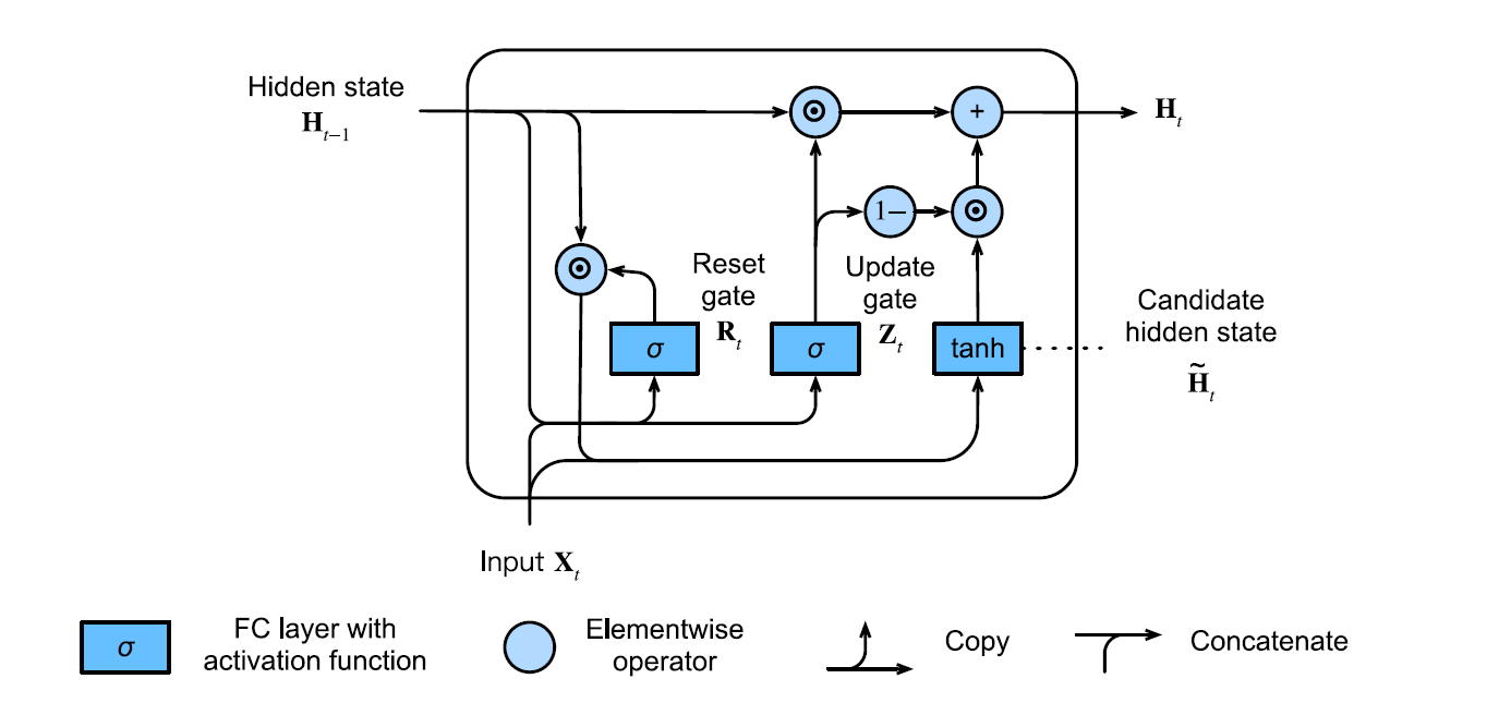
• The Gated Recurrent Unit (GRU) offers a more streamlined version of the LSTM. It improves memory cells computationally without sacrificing performance

• Let be the number of examples be the number of inputs. be the number of hidden units. be the input as a minibatch be the hidden state - sigmoid activation

• We replace the three gates with only two.

  • Reset Gate - controls how much of the previous state wee remember. It captures short-term dependencies in the sequence.

    The reset gate is computed as

    Where and are weights, and is a bias parameter.

    • When is close to we recover a vanilla RNN.
    • When is close to , we have an MLP with as input and any pre-existing hidden state is reset to their defaults.

  • Update Gate - controls how much of the new state is just a copy of the old state. It captures long-term dependencies in the sequence.

    The update gate is computed as

    Where and are weights, and is a bias parameter.

    • When is close to , we retain the old state. Any information from is ignored and we skip time step .
    • When is close to , the new hidden state approaches the latent state .

GRU cell. Image taken from Zhang et al.

• We first derive a candidate hidden state using only the reset gate as follows

  Where and are weight parameters and is the bias term. We also use the Hadamard product and the activation function.

• The hidden states are calculated using the update gate

• In the derivation of the candidate hidden state, rather than performing matrix multiplication to model the influence of previous hidden states, we can instead reduce this to performing elementwise multiplication.

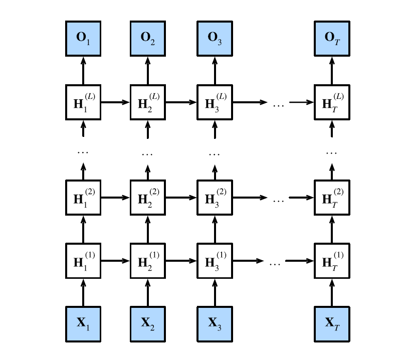
Deep RNN §

• A Deep RNNN is a variant which involves using multiple recurrent layers stacked on top of each other.

• Given a sequence of length , one layer produces a new sequence of the same length and this is fed to the next layer.

• *Each hidden state operates on a sequential input and produces sequential output. *

• Any RNN cells at each time depend on both the same layer’s value at the previous time step, and the previous layer’s value at the same time step.

• More formally, Let be the size of a minibatch be the number of inputs in each example be the number of layers in the network. be the hidden state at the -th layer. be a minibatch of inputs (i.e., we treat the input as the -th layer). be some activation function

  Then

  Where and are weights ,and is a bias term.

  The output layer is calculated as

  Where is the weight and the bias is . These are parameters of the output layers.

Deep RNN. Image taken from Zhang et al.

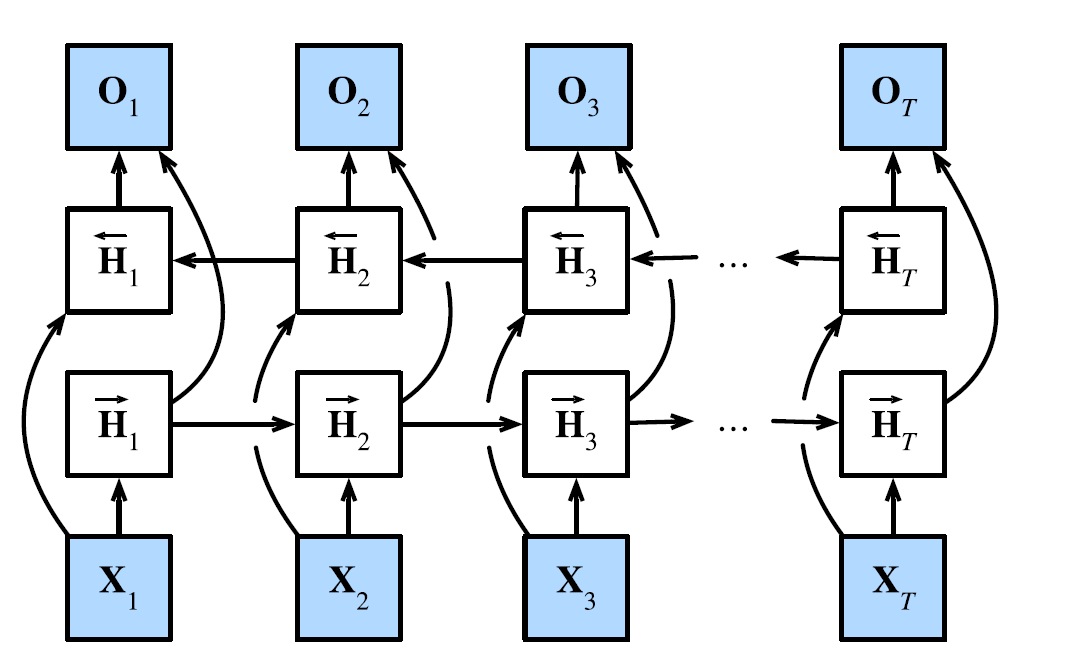
Bidirectional RNN §

• A Bidirectional RNN is a variant of an RNN which is a combination of two RNNs training the network in opposite directions. One starts from the beginning of a sequence, while the other from the end of a sequence.

  • The bidirectional RNN is motivated by allowing the model to learn from future events as well. This provides additional input information available to the network.
  • This is especially useful when the context of the input is needed, i.e., for a particular data point, we need to look at the temporally local data points.

• Let be the number of examples be the number of inputs in each example be the number of hidden units. be the number of outputs. be the activation function be a minibatch input. be the forward hidden state be the backward hidden state. be the output of a layer.

  We update the hidden states as follows:

  Where we have weight parameters and bias parameters.

  Then, we concatenate the forward and backward hidden states to obtain the hidden state .

  In a deep BRNN with multiple hidden layers, the hidden layer state is passed as input to the next bidirectional layer.

  We then calculate the output layer as

Bidirectional RNN. Image taken from Zhang et al.

RNN Encoder Decoder §

• See Encoder-Decoder Network.

Links §

• Recurrent Neural Network
• Dive into Deep Learning by Zhang, Lipton, Li and Smola