Dynamic Programming for Reinforcement Learning

Dynamic Programming §

• Generally Dynamic Programming methods follow the process of bootstrapping where they update estimates are based on other estimates.
• DP performs expected updates where the estimates are based on the complete distribution of successors.
• These methods assume perfect knowledge about the environment—particularly the states, their transitions and their rewards.

Bellman Equations §

• The value function of a reinforcement learning task modelled as an MDP can be quantified recursively using the Bellman Equations (see here)

  • The value of the current state must equal the immediate reward plus the discounted value of the expected next state. This is also called a Bellman Backup.
  • Note that backups can be performed on the optimal policy as well.

• Optimal Policies satisfy the following properties (from the optimal Bellman equation)

  • The value of a state under a policy must equal the expected return for the best action from that state.
  • The value of an action given a state under a policy is equal to reward for the action plus the expected return for the next state.
  • The value for both is the same across all optimal policies.
  • Greedy policies are optimal as long as we have the optimal value functions or .

Policy Evaluation §

• Iterative policy evaluation involves the use of approximate value functions and the Bellman equation as an update rule.

  • The approximate value function is obtained iteratively through one full backup That is, starting with an arbitrary (except for terminal states which are initialized to ), obtain by performing a backup using the previous approximation

• Policy Improvement Theorem: Let and be deterministic policies such that ,

  Then the policy must be as good as or better than , or

  Moreover, this result is monotonic.

  • A switchable state is a state for which such that .
  • Optimal policies do not have switchable states

Policy Iteration §

• The optimal policy in an MDP can be obtained through policy iteration wherein the policy is incrementally improved until its value function can no longer be improved. This method is supported by the policy improvement theorem.
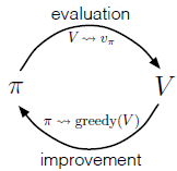
  • Generally this consists of two phases of evaluation and improvement.
    • Evaluation consists of computing the value function for a policy.
    • Improvement consists of giving an improved policy given the value function.
  • We evaluate each action taken on each state using the Q-Function. We then form a new policy by considering all states and greedily taking the actions that do well on each state.
    • In case of a tie, we need only ensure that all the suboptimal policies are given probability. That is, the new policy is evaluated on state as
  • This method of policy iteration is guaranteed to monotonically converge to the global optimum (for a proof of why see Sutton and Barton Ch. 4.2).
  • This process is guaranteed to stop assuming a finite MDP. This is because the value of the policy always monotonically increases, and there are only finitely many policies.

Value Iteration §

• A variation of policy iteration is called value iteration wherein we no longer perform a full backup in policy evaluation. This tends to be more efficient as it combines policy iteration and evaluation steps in one pass.
  • This is done using a simple update function done as follows:
  • It combines policy evaluation and one step of Policy Iteration, leading to faster convergence.

Generalized Policy Iteration §

• Generalized Policy Iteration refers to the general idea of letting policy-evaluation and policy improvement processes interact. As long as all states are continually evaluated and updated (that is updated an infinite number of times), convergence is guaranteed.
  • This process can be viewed in adversarial light. Changes in the value will make the policy wrong and vice versa. However, they both converge to both an optimal value and an optimal policy.
  • The value function stabilizes only when it is consistent with the current policy, and the policy stabilizes only when it is greedy with respect to the current value function

GPI. Image from Sutton and Barto (2017)

Optimizing DP §

• It should be noted that DP is already quite efficient as it is. It takes polynomial time to complete which is much faster than the exponential time to search through the whole state space.

• Asynchronous Dynamic Programming is a method where instead of performing systematic sweeps over the state set, backup is performed in any order using the values that happen to be available.

  • Caveat: all states must be used in the backup process. States must not be continually ignored..
  • This can be used on problems where the agent is expected to learn in real time.
  • It is also important when considering memory constraints.

• Another method is to evaluate the states that are to be backed up such that convergence is achieved much faster.

• Real Time Dynamic Programming is an on-policy trajectory sampling version of value iteration.

  • Unlike other on-policy methods (such as SARSA), this approach does not require the assumption of Exploring Starts. That is, we need not visit states (especially those that are uninteresting) infinitely often.
  • This works when we have undiscounted episodic tasks using an MDP with absorbing goal states that generate 0 reward. And provided that we have a stochastic optimal path problem.
    • The initial value of every goal state is
    • There is at least one policy that guarantees that a goal state will be reached with probability from any start states.
    • All rewards for transitions on non-goal states are strictly non-negative.
    • All initial values are their optimal values.

Stochastic Games §

• DP can also be used for Stochastic Games. The update rule is for a minimax solution to the non-repeated normal-form. Denote this by for agent and state

• After updating all possible ’s we can update the value function of the -th agent

  Where is the minimax value for agent .

• This reduces to the usual Bellman equations in the single-agent case

Links §

• Markov Processes in Machine Learning - for an overview of MDPs

• Sutton and Barto Ch. 3.7 - 3.9, Ch. 4 - discussion on value functions and the Bellman Equation and approximately optimal solutions.

  • 4.1 - for Policy Evaluation
  • 4.4 - for Value Iteration
  • 8.7 - Real Time DP

• Albrecht, Christianos, and Schafer - Ch. 6.1

• Stanford CS234

  • At time 55:55, the Policy Improvement Theorem is explained.