Factory Optimization Techniques

• We can optimize throughput as follows:

  • *Increase bottleneck rate *
  • Increase bottleneck utilization by reducing blocking and starving.
    • Buffer the bottleneck with WIP by increasing the buffer size of the system (either by expanding it or reducing queue times). For maximum effect, we should prioritize the spaces immediately in front of and immediately after the bottleneck
    • Buffer the bottleneck with capacity by increasing the effective rates of non-bottleneck stations. Generally, we want to target the highest utilization non-bottleneck station
      • Faster stations upstream make starving less frequent.
      • Faster stations downstream make blocking less frequent.

• In a system where setups are long but processes are close together, it might make good sense to keep process batches large and transfer batches small. This practice is called lot splitting and can significantly reduce the cycle time

• We can use large process batches in conjunction to setup time reduction to keep utilization, cycle time and WIP under control

• If setup times can be made sufficiently short, then using serial batch sizes of one can reduce cycle times. Otherwise, cycle time is sensitive to process batch size

• For parallel batch operations, the cycle time is significantly affected by batch size.

• We can optimize cycle time as follows.

  • Reduce queue time — queue times are caused by utilization and variability so we have two options for policies
    • Reduce utilization by increasing the effective rate at the bottleneck (either increasing bottleneck rate or reducing flow into the bottleneck)
    • Reduce variability in either process times or arrival times, prioritizing high-utilization stations.
  • Reduce process batch time which is driven by the choice in process batch size.
    • Batch optimization to balance batch time with queue time due to high utilization.
    • Setup reduction to allow smaller batches without increasing utilization.
  • Reduce Wait to match time which is driven by a lack of synchronization of component arrivals at an assembly station.
    • Fabrication variability reduction to reduce the volatility of arrivals to the assembly (i.e., by reducing queue times)
    • Release synchronization using scheduling techniques and shop floor control.
  • Increase Station overlap time using lot splitting or streamlined material handling (via cellular manufacturing)

• *Satisfying customer needs is primarily about lead time (quick response) and service (on-time delivery).

  • We should favor make-to-stock systems rather than make-to-order.
  • Alternatively, we can make generic components to stock and assemble to order.
  • The main driver for lead time is the cycle time, so reducing cycle time also helps reduce lead time.

• Improving a manufacturing system is not simply a matter of removing constraints. There is also a people aspect to consider.

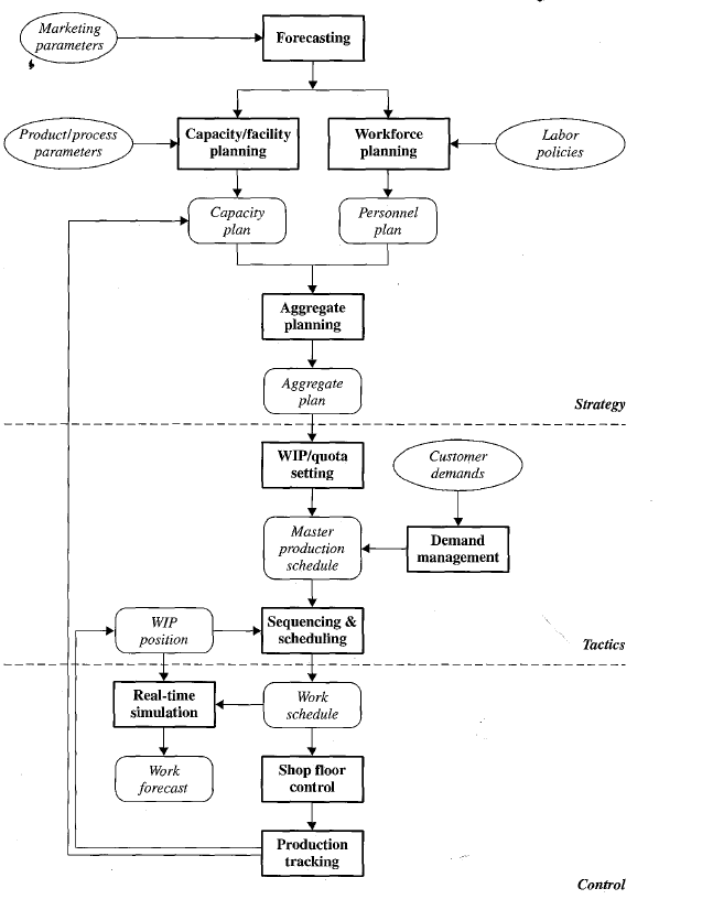
Planning Framework §

• Problems at different levels of the organization require different levels of detail, modeling assumptions and planning frequency

• Planning and analysis tools must be consistent across levels. A planning framework has the following steps [^planning]

  • Divide the system appropriately in both temporal and spatial scales. Wider planning horizons require lower level of detail.
  • Identify links between the divisions. The links should be simple.
  • Use feedback to enforce consistency. However, this is often offset by the distributed nature of the production line.

• We can disaggregate the entire production system across different time and spatial scales.

• In the temporal scale, we can divide the planning horizon broadly into long (strategic), intermediate (tactical) and short (control) scales.

Time Horizon	Representative Decisions
Strategy	Financial Decisions Marketing Strategies Product Designs Process Technology Decisions Capacity Decisions Facility Locations Supplier Contracts Personnel Development Programs Plant Control Policies Quality Assurance Policies
Tactics	Work Scheduling Staffing Assignments Preventive Maintenance Sales Promotions Purchasing Decisions
Control	Material Flow Control Worker Assignments Machine Setup Decisions Process Control Quality Compliance Decisions

• We can categorize various aspects of the plant as follows:
  • Processes
  • Products
  • People

Forecasting §

• First Law of Forecasting: Forecasts are always wrong.

• Second Law of Forecasting: Detailed forecasts are worse than aggregate forecasts.

• Third Law of Forecasting: The further into the future, the less reliable the forecast.

• Decisions are made using forecasting. These decisions should be robust with respect to forecasted estimations.

• In any forecasting environment, situations will arise in which the forecaster must override the quantitative model with qualitative information.

• Quantitative Forecasting is based on the assumption that the future can be predicted using numerical measures of the past in some mathematical model.

  • Causal Models - predict a future parameter as a function of other parameters. ¹
  • Time Series Models - predict a future parameter as a function of past values of that parameter.

Pull Planning §

• Pull systems are harder to plan for because they are rate driven. It is hard to know the actual rates until the system is ran.

• The conveyor model of Cycle Time is an improvement over MRP’s model of fixed cycle time. The time to process a quantity of WIP is dependent on the capacity of the line.

  Where represents the time a job can go through an uncongested line, and represents the capacity of the line

  • It is based on the observation that pull systems maintain fairly steady WIP levels, so the speed of the line is constant.

  • The line can be parameterized with the practical production rate and the minimum practical lead time which indicate the anticipated throughput and minimum lead times.

    We have that

    The time a job is completed is then provided by

• Capacity / Facility Planning concerns how much and what kind of equipment to purchase, how to lay out, staff, power, and support them. It also concerns

  • Product Lifetimes - how long do we anticipate making the product. This influence capacity.
  • Vendoring Options - do we make or buy certain products and components. We can note the following
    • It is not solely dependent on cost.
    • Consideration should be given to the long term.
    • When the make-or-buy decision concerns whether or not to make the product at all, then it is clearly a capacity planning decision
  • Pricing - a valid economic analysis should take into account the price of products.
  • Time Value of Money - capital generally means better capacity and equipment. We should take into account interest and depreciation rates.
  • Reliability and Maintainability - all things being equal, we want mean time to failure to be big and mean time to repair to be small.
  • Bottleneck Effects - capacity increases at bottleneck resources typically have a larger effect on throughput.
  • Congestion Effects - variability degrades performance, so we should also consider non-bottleneck resources.

• Workforce Planning - determines what workforce is needed to support production., considering how much and what kind of labor is available as constrained by labor policies. We should take into account the following

  • Worker availability - take into account leave and training time that reduce worker availability.
  • Workforce stability - a firms’ ability to recruit qualified people, and its overall workplace attitude, can be strongly affected by changes in the size of the workforce.
  • Employee training - training new recruits costs money and takes the time of current employees.
  • Short term flexibility - workforce planning needs to look beyond the production plan to consider the unplanned contingencies with which the system can cope.
  • Long term agility - the workforce is a key source of agility — allowing the plant to reconfigure the system for efficient production.
  • Quality improvement - establishing quality oriented techniques should be incorporated to workforce planning.

• Aggregate Planning specifies how much of the product to produce over time subject to constraints ²

• WIP/Quota Setting translates the aggregate plan to control parameters.

  • WIP setting - we do not need complex models for WIP levels. We only need to set a desired WIP level. Adjustments to WIP should be done infrequently to ensure adjustments are done based on long-term estimates.

    The WIP level can be set by taking into account a desired cycle time, and the practical production rate

  • Quota setting means establishing a periodic quantity of work that we will almost always complete during the quota period. This means

    • Production during the period stops when the quota is reached.
    • Overtime is used at the end of the period to make up any shortage that occurred during regular time.
    • We can achieve a steady output

  • Quota setting should take into account cost and capacity .

• Demand Management allows us to filter and adjust customer orders that produces a manageable MPS. This gives us control of the environment by smoothing out production for a smoother rate..

  • Demand management should take into account manufacturing capabilities.

• Sequencing provides a schedule that governs release times of work orders and materials and then facilitates their movement through the factory.

• Shop Floor Control uses the work schedule as a source of general guidance — adhering when possible and adjusting when necessary.

• Real time simulation using simplified models provides a good tool for analysis, diagnosis, and optimization.

• Production Tracking is responsible for tabulating and displaying data regarding production, especially operations which failed.

Shop Floor Control §

• A well-designed SFC module both controls the flow of material through the plant and makes the rest of the production planning system easier to design and manage
• We have the following elements and considerations
  • Gross capacity control. We want to set up lines to run at a steady pace by matching capacity with demand We have the following options:
    • Vary the number of shifts.
    • Vary the number of work days or hours - establish planned overtime.
    • Vary the level of staffing. Add workers as needed to increase capacity.
    • Use outside vendors to mitigate some demand variability
  • Bottleneck Planning. We not only want to control the utilization of the bottleneck, but also identify this bottleneck process to begin with. Sometimes, especially for multiproduct lines, the bottleneck for one product is not the bottleneck for another.
    • Stable bottlenecks are easier to manage.
    • Bottlenecks can be designed.
  • Span of Control pertains to the number of employees or products under direct supervision of the manager.
    • The SFC module must tell managers what parts are required by downstream workstations.

SFC With CONWIP §

• A CONWIP system for SFC is suitable when —

  • There are constant routings so all parts traverse the same sequence of machines (or additional operations that do not alter flow time).
  • Processing times are similar so all parts require roughly the same amount of time at each process center.
  • There are no significant setups so the time through the line for an individual job is not strongly affected by the sequence of jobs.
  • There are no assemblies so we can view the progression of jobs as a linear flow.

• Some issues to consider and resolve

  • Because the CONWIP cards do not contain product information, a line manager or operator needs additional information to select jobs to release into the line. This allows us to keep track of work backlogs
  • The line must maintain a FIFO order (barring rework). We want to minimize expediting that can disrupt the lines to establish line discipline
    • To minimize such disruptions, we can establish specific passing points between CONWIP loops where hot jobs are allowed to pass normal jobs.
  • SFC must fix a reasonable WIP level.
  • We can maintain WIP deficits to allow jobs to bypass the CONWIP system. This will allow us to regulate our WIP level.
  • Work ahead when opportunity arises. We should establish a work-ahead window where we do this.

• We can consider Tandem CONWIP lines when we want to decouple the line into multiple manageable parts.

  • One tradeoff is between efficiency vs span of control (more lines = more efficiency but less span of control)
  • Another consideration is the added complexity to the system.
  • Having tandem CONWIP lines lets one line do work ahead independently of other lines. This is relevant for bottleneck loops.

• Shared resources complicate the use of CONWIP lines because we must choose a job from multiple incoming routings. The proper way is to use First-in-System, First-Out

• Shared resources also complicate prediction because of the added complexity in the system. This can be mitigated by using

• If we have multiple product families, it becomes more difficult to control the WIP level of the line. Automated systems (i.e., using computers) would be required to manage the system.

• If we have multiple assemblies, longer input lines become the bottlenecks. Assuming lines have sufficient WIP to prevent starvation of the bottleneck, the performance is robust to WIP level.

Pull Systems §

• We can use Kanban (single station loops) instead of CONWIP

  • This offers the following advantages
    • It forces better interstation communication by causing stations to pull upstream.
    • It provides easier mechanisms for resource sharing across different routings.
  • This has the following disadvantages
    • More complicated than CONWIP
    • It requires tighter pacing leading to less flexibility.
    • At least one standard container for each part number must be maintained at each station.
    • It cannot accommodate a changing product mix
    • It is impractical for small, infrequent orders. Either WIP will be left unused or the system will be inflexible.

• We can use Pull from the Bottleneck methods. Here the bottleneck can work ahead but not too far ahead

  • This offers the following advantages.
    • It mitigates bottleneck starvation due to downstream machine failures.
    • It mitigates premature releases due to WIP levels being constant.
  • The goal is to ensure that jobs are released so they arrive at the bottleneck at a specified time before they are needed.
    • This naturally forms a buffer that prevents random variations from causing the bottleneck to starve.
    • If jobs wait on average units at the bottleneck, and is large enough, the work sequence at the bottleneck should match the sequence on the work backlog.

• Adding scheduling to SFC would enable us to prevent WIP from exploding.

Production Tracking §

• Statistical Throughput Control concerns itself with short term control. In particular, we want to make sure that we are on schedule.

  • Starting at time and operate on a period . We compare the following information

    - actual cumulative production by line in time interval . - scheduled cumulative production for line for time interval .

    Ideally we want

    But variability can make this hard to compute, in addition to not providing information about the risk of being behind schedule. Hence we may be more interested in the probability of being on schedule by the end of the regular time period given how far ahead or behind we are now

  • increases monotonically, while can potentially decrease due to yield loss.

  • If the line uses a detailed schedule, increases unevenly.

  • If the line uses periodic schedules (i.e., with quota ), then we assume

    • If we assume the production follows a normal distribution of mean and standard deviation of and , we can compute

      Where obtained from the standard normal table.

      The following holds

• Long Range Capacity Tracking concerns itself with providing input to other planning functions based on key data from regular time production of the plant.

  In particular, we want data for the time to make quota and then apply techniques from Time Series Analysis to determine the long term trend.

Production Scheduling §

• Production scheduling aims to accomplish the following:

  • Meet due dates — whether it be customer due dates or material requirements.
  • Maximize Utilization
  • Reduce WIP and Cycle time.

• Scheduling is a difficult problem. Even models that aim to solve or simulate scheduling may fail to consider the following

  • The plant may have multiple machines
  • Process times are not deterministic
  • All jobs are not ready at the beginning of the problem , and instead continuously arrive.
  • Process times are frequently sequence dependent.

• However, while scheduling is difficult, we can frame the problem as one involving environmental control.

  • We can control the due dates.
  • We can split jobs so that we have large process batches and small move batches.
  • Rather than aim for optimal schedules, we aim for good, feasible schedules.
  • Focus on scheduling jobs for bottleneck areas.
  • Use capacity control mechanisms.

• Generally, we have two approaches

  • Simulation-Based Scheduling - we create a simple model and simulate it to obtain expected job arrival and departure times at each station. We then use dispatching rules to dictate different schedules.
    • It is easy to explain and can quickly generate a variety of schedules.
    • It is not without its downsides
      • It is data hungry
      • It may not account for variability and so may not be entirely accurate
      • It is more of a trial and error process so there is no guarantee of optimality.
      • If we are building on top of an infeasible schedule, a simulation based approach will not make it feasible.
  • Optimization-Based Scheduling - we use heuristic procedures with guarantees for performance.

• Ideally, planning and scheduling should be coupled together. Planning should not produce an infeasible schedule as a result of not considering capacity or throughput.

  • One remedy to the disconnect between planning and scheduling is the reduction of cycle time.
  • We can choose an appropriate batch size

    • For serial batches with one product, a good batch size can be obtained by

    • For serial batches with multiple products in the mix, a good batch size can be found as follows. Let be the number of products, indexed by .

      Define

      Where denotes the station utilization time without setups.

      The optimal batch size for the -th product is

    • For parallel batches, we want to balance effective capacity utilization (large batches) and minimal wait-to-batch time (small batches)

      Define

      Where is the utilization from having a batch size of .

      When is sufficiently small, we can approximate the above as

      The optimal batch size is
  • Another approach to scheduling is to properly quote our due dates. The difficulty in this solution lies in accounting for manufacturing and personnel.

Aggregate Planning §

• The goal is to decide what the plant will produce. This decision affects other aspects such as staffing, supply, and marketing.

• The model depends on the business needs.

• One important input is the forecasted demand.

• A simple model involves solving the following.

  Let - be the profit per unit product sold be the quantity produced during period assumed available to satisfy demand be the quantity sold. Unsold units are assumed available still be the inventory.

  We optimize the following

• An extension of the simple model considers multiple product mix’

  Denote the time for the -th workstation to produce one unit of product .

  - the time required on workstation to produce one unit of product . be the capacity of the workstation the net profit of product

  - the maximum demand for product . - the minimum demand for product

  We optimize the following

  • We can extract the following from the more comprehensive model
    • The demand feasibility determines whether a set of demands is capacity feasible (i.e., if is tight)
    • The bottleneck locations are determined using the second constraint above. If a workstation limits capacity at certain periods, it becomes a bottleneck.
    • The product mix is determined by balancing capacity with the ability to meet demand, and the ability to turn a profit.
  • The model can be extended in a variety of ways.

    • Use resource constraints

      Let be the number of resource per product be the number of units of resource available in period be the amount of product produced in period

      We have

    • Use utilization matching. This addresses two issues - the low granularity of an aggregate planning module, and incorporating other production control decisions to aggregate planning.

      If experience dictates, it is reasonable to run percent of full capacity, then we replace the second constraint with

    • Incorporate Backorders by removing the implicit assumption that inventory remains positive at all times.

      We do this by maximizing the new objective

      adding the constraint

      Where represents the inventory carried over from period to for product represents the number of backorders carried from to . represents the penalty of carrying one unit of product on backorder for one period of time

      Here we refer to as the inventory position.

      • Typically is adjusted relative to depending on what is needed.
      • High values tend to force the model to build inventory
      • Low tends to allow the model to be late in satisfying some demands.

Workforce Planning §

• This encompasses both high-level planning (how many to hire, how to train them) and low-level planning (when to hire / fire, when to schedule training).
• Low-level planning is based on the aggregate plan.

Links §

• Hopp and Spearman
  • Ch. 13 - discussion on planning frameworks
  • Ch. 15 - scheduling frameworks. Derivations for optimal batch sizes are found in this chapter.
  • Ch. 16 - aggregate and workforce planning
• Fundamental Objects in Factory Physics
• Factory Dynamics
• Factory Variability

Footnotes §

1. A good example is linear regression ↩

2. We can do this with something like Linear Programming ↩