Adaptive Transformer

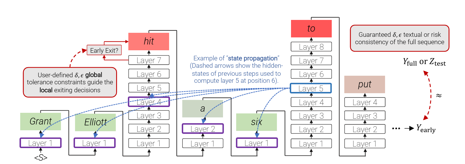
• ¹ proposes Confident Adaptive Language Modeling (CALM) which is a calibrating method that dynamically allocates different amounts of compute per input and generation timestep.

  • Early exiting is a promising approach to decreasing the computational cost of multilayered architectures

    • CALM extends this by scoring and assigning “consistent early-exit” confidence scores after each layer. The decision to exit is calibrated using a calibration set.

  • One metric is via textual consistency Given a bounded text dissimilarity function and a calibration set , where each is a prompt, we aim to calibrate the early exiting LLM such that its predictions agree to a tolerance with the full model in expectation with high probability

    • An adaptive LLM is textually consistent if given any bounded and tolerance , .
    • This is doable with unlabeled calibration data.
    • The disadvantage of the above is that it may be unnecessarily strict for certain tasks.

  • We can also enforce risk consistency using prompts paired with target references . The calibration set and any bounded risk function gives us the following objective

    • An adaptive LLM is risk consistent if given any and tolerance .

  • For the above implicitly, and are assumed to be normalized between so that .

  • We choose by computing where is the layer output of the -th layer.

    Let denote a confidence score for layer , token . Let denote an early exiting threshold.

    The model exits early if . Otherwise, it compute the next representation.

    If the model has early exited at some layer for a token then is not available. An approximation is to perform state copying we set for all layers .

    • Experiments show that the model is robust to state copying from lower layers.
    • Experiments also show that we can save compute without impacting performance given a good confidence measure.

  • Training is done for local consistency since training for global consistency could be challenging.

    The training objective is defined as the weighted average of losses for each layer. We set to be the negative log-likelihood loss to obtain

    Where is configured to favor higher layers.

  • We have a few choices for confidence measures.

    • Softmax Response - take the difference between the top two values of the output logits.
      • Disadvantage: Many FLOPs for large output vocabularies.
      • Advantage: Next layer can start its computation in parallel.
    • Hidden State Saturation - take the cosine similarity between and .
      • Advantage: Parameter free and fast.
      • It identifies early saturation events of the hidden state.
    • Early Exit Classifier - train a linear classifier to predict the likelihood of exiting with local consistency given the hidden state.

  • To choose we make use of the Learn-Then-Test calibration framework from ².

    • We obtain the -values for the framework using the empirical consistency of the early-stopping LLM measured over a random calibration sample and using Hoeffding’s inequality.
      Where and depends on our consistency metric.
    • For textural consistency
    • For risk consistency

CALM generation. Image taken from Schuster et al. (2022)

• ³ proposes Depth Adaptive Transformer which can adjust the amount of computation performed per time step.
  • Rationale: Large scale models are overkill for small-scale generation tasks. Prior methods apply the same amount of computation ignoring the required output scale.
  • It extends Adaptive Computation Time (ACT) ⁴ and Universal Transformers ⁵.
    • The model includes mechanisms to estimate network depth and applies a different layer each step.
  • It also borrows from Anytime Prediction where predictions can be done at different layers.

    • We attach output classifiers to the output of each of the decoder blocks. Each classifier is parameterized by and we obtain an intermediate output as follows

    • Dynamic computation means we can use any of the classifiers as exit points, which we denote . We denote the exit point for the decoder as

    • We have two options for training.

      • Aligned Training - all classifiers are optimized simultaneously.

        • We assume that all previous hidden states are available.

          The loss function per exit is then

          And the total loss is the weighted average of each .

        • At test time, the assumption fails. We instead copy the last computed state to all upper layers (with layer specific KV projections applied first).

      • Mixed Training - we sample several sequences of exits and expose the model to hidden states from different layers.
        • Suppose we sample exit sequences . We use the following loss
          With the decoder loss being the average of the above across all sequences.

    • The distribution of exiting at time step is modeled with a parametric distribution . The parameters of are optimized to match an oracle via cross entropy loss backpropagated to the encoder-decoder parameters.

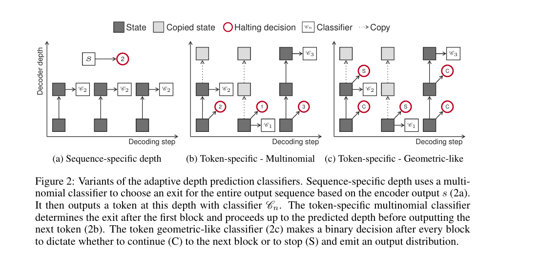
    • To perform adaptive depth estimation, we consider two options.

      • Sequence specific depth decodes all outputs using the same block.
        • Let and be parameters for the halting mechanism. and be the encoder output at time . We model as follows
      • Token specific depth chooses a different exit at every time step. We have two approaches for
        • Multinomial
          With the most probable exit chosen at inference.
        • Geometric-Like
          During inference, the decoder exits when the halting signal exceeds a hyperparameter (or if not exceeded, exit in the last block as normal)

    • Our choices for the oracle are as follows:

      • The likelihood of the entire sequence modeled with a Dirac Delta regularized to encourage lower exits that achieve good likelihood

        This ignores whether the model already assigns the highest score to the correct target

        For Token-Specific Depth, we also smooth likelihoods with an RBF kernel since we ignore the impact of the current decision on future time steps.

      • Correctness based. Here we choose the block with the most number of correct tokens at time step (and for Token Specific Depth, also the surrounding tokens)

Adaptive Depth Prediction. Image taken from Elbayad, Gu, Grave, and Auli (2019)

• ⁶ proposes a self-attention mechanism that can learn its optimal attention span

  • Rationale: Attention is costly, especially for large context windows.

  • Each head independently learns its attention span .

    For each head, we add a masking function to control the span of attention. The masking function normalizes distance (i.e., it is of the form ).

    Our choice of function is the following (parameterized by )

    Where is a hyperparameter controlling softness.

  • The attention weights are computed with the masked span as follows

  • We add an L1 penalty on the parameters for each attention head of the model to the loss function

  • To extend it further, we can make a function

    Where are learnable parameters.

  • Result: Lower layers do not require long attention spans. Higher layers may use longer attention spans.

  • Adaptive attention span can reduce the number of FLOPs.

Links §

• Transformer Model

Footnotes §

1. Schuster et al. (2022) Confident Adaptive Language Modeling ↩

2. Angelopoulos et al. (2021) Learn then Test: Calibrating Predictive Algorithms to Achieve Risk Control ↩

3. Elbayad, Gu, Grave, Auli (2019) Depth Adaptive Transformer ↩

4. Graves (2016) Adaptive Computation Time for Recurrent Neural Networks ↩

5. Deghani et al. (2019) Universal Transformers ↩

6. Sukhbaatar, Grave, Bojanowski, and Joulin (2019) Adaptive Attention Span in Transformers ↩